---
title: "Disaster Death Distributions: 1950-2020"
subtitle: "How the patterns of mortality from natural disasters changed over time"
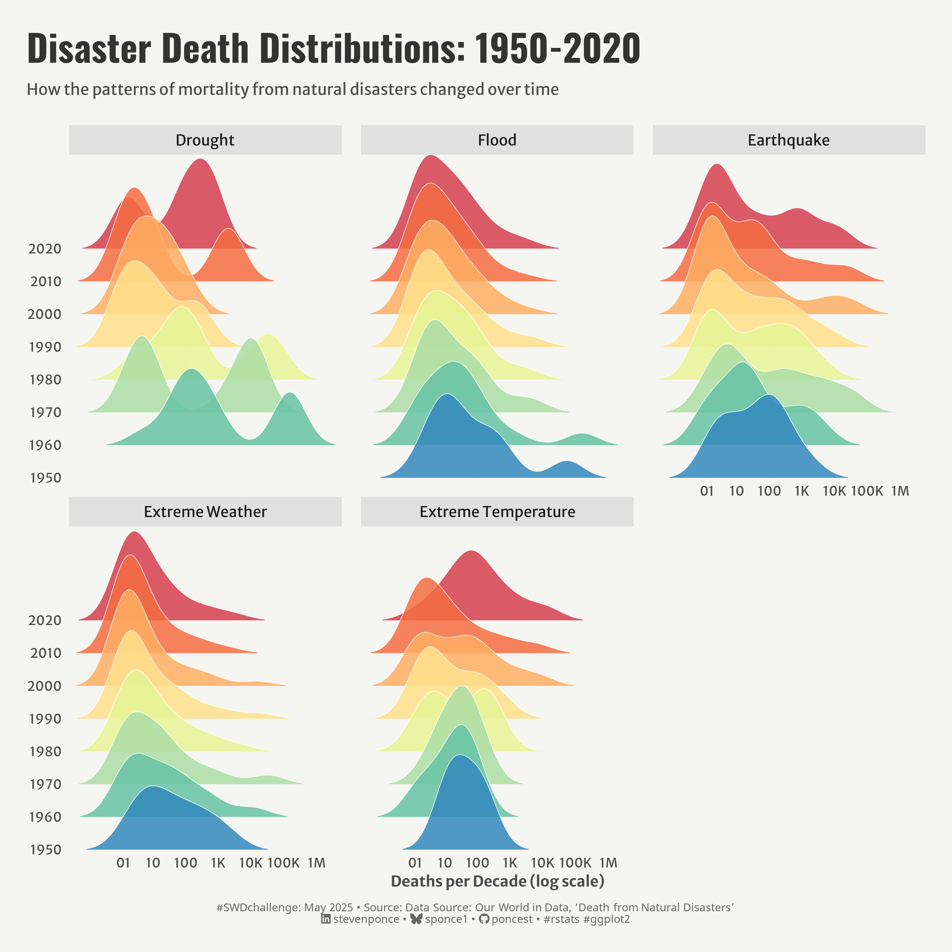
description: "This visualization explores the evolving patterns of natural disaster-related deaths from 1950 to 2020 using ridgeline plots. The analysis reveals how mortality distributions have shifted across five major disaster types: drought, flood, earthquake, extreme weather, and extreme temperature."
author: "Steven Ponce"
date: "2025-05-02"
categories: ["SWDchallenge", "2025"]
tags: [
"ridgeline plots", "natural disasters", "mortality patterns", "ggridges", "temporal analysis", "distribution visualization", "log scale", "disaster trends", "environmental data", "public health", "AI", "claude.ai"
]
image: "thumbnails/swd_2025_05.png"
format:
html:
toc: true
toc-depth: 5
code-link: true
code-fold: true
code-tools: true
code-summary: "Show code"
editor_options:
chunk_output_type: inline
execute:
freeze: true
cache: true
error: false
message: false
warning: false
eval: true
# share:
# permalink: "https://stevenponce.netlify.app/data_visualizations/SWD Challenge/2025/swd_2025_05.html"
# description: "Exploring seven decades of natural disaster mortality distributions through innovative ridgeline plots. See how death patterns from droughts, floods, earthquakes, and extreme weather events have evolved over time."
# linkedin: true
# twitter: true
# email: true
---
### Original
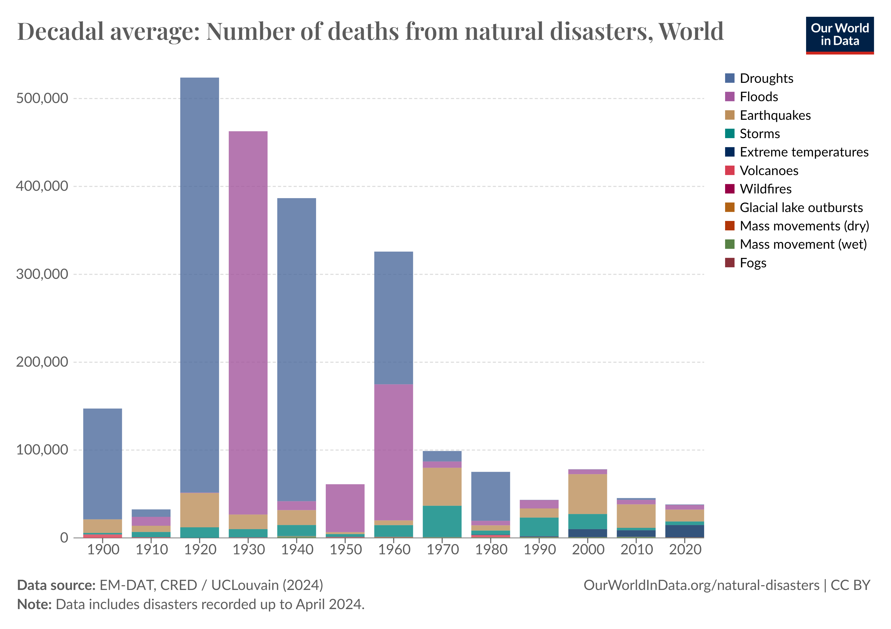
This month's Storytelling with Data exercise aims to find a graph or slide that is ripe for improvement. Consider what you want to improve within the visual and implement those changes. Then, select an AI tool that can create visuals from prompts and a starting image. Ask the tool to consider the original image and prompt it to outline potential improvements.
{#fig-1}
Additional information can be found [HERE](https://community.storytellingwithdata.com/challenges/may-2025-compare-human-vs-machine)
### AI (claude.ai)
**Prompt Title:** Improve this chart on natural disaster deaths
**Prompt:**
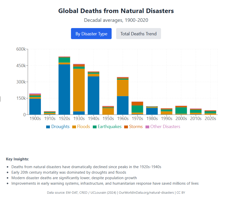
This is a historical stacked bar chart showing the decadal average number of deaths from natural disasters globally, segmented by disaster type (e.g., droughts, floods, earthquakes). The original chart is from Our World in Data and spans from 1900 to 2020.
Help redesign this visual to improve clarity, storytelling, and visual appeal. Please:
- Simplify the visual by reducing clutter and using a limited, colorblind-friendly palette.
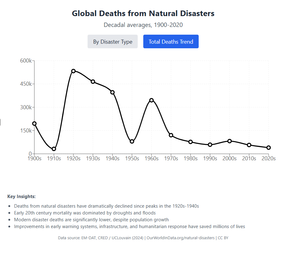
- Highlight major insights, like the sharp decline in deaths over time and changing causes.
- Use modern fonts, consistent scales, and clear legends.
- Create a layout that is easy to read and suitable for a web article or presentation.
Output a cleaner, more engaging visual that tells the story effectively to a broad audience.
**Chat link:** https://claude.ai/chat/e8de4711-f7b5-4f82-b128-3a7f3568cc3f
::: {layout-ncol=2}
{#fig-2}
{#fig-3}
:::
### Makeover
{#fig-4}
### <mark> __Steps to Create this Graphic__ </mark>
#### 1. Load Packages & Setup
```{r}
#| label: load

if (!require("pacman")) install.packages("pacman")
pacman::p_load(
   tidyverse,         # Easily Install and Load the 'Tidyverse'
  ggtext,            # Improved Text Rendering Support for 'ggplot2'
  showtext,          # Using Fonts More Easily in R Graphs
  scales,            # Scale Functions for Visualization
  glue,              # Interpreted String Literals
  here,              # A Simpler Way to Find Your Files
  janitor,           # Simple Tools for Examining and Cleaning Dirty Data
  skimr,             # Compact and Flexible Summaries of Data
  ggridges,          # Ridgeline Plots in 'ggplot2'
  RColorBrewer,      # ColorBrewer Palettes
  camcorder          # Record Your Plot History
)

### |- figure size ----
gg_record(
  dir    = here::here("temp_plots"),
  device = "png",
  width  = 10,
  height = 10,
  units  = "in",
  dpi    = 320)

# Source utility functions
suppressMessages(source(here::here("R/utils/fonts.R")))
source(here::here("R/utils/social_icons.R"))
source(here::here("R/utils/image_utils.R"))
source(here::here("R/themes/base_theme.R"))
```
#### 2. Read in the Data
```{r}
#| label: read

deaths_disasters_type_raw <- read_csv(
  here::here("data/MakeoverMonday/2025/decadal-deaths-disasters-type.csv")) |>
  clean_names()
```
#### 3. Examine the Data
```{r}
#| label: examine
#| include: true
#| eval: true
#| results: 'hide'
#| warning: false

glimpse(deaths_disasters_type_raw)
skim(deaths_disasters_type_raw)
```
#### 4. Tidy Data
```{r}
#| label: tidy

# Pivot longer
deaths_long <- deaths_disasters_type_raw |>
  pivot_longer(
    cols = starts_with("deaths_"),
    names_to = "disaster_type",
    values_to = "deaths"
  ) |>
  # Clean disaster type names
  mutate(
    disaster_type = str_remove(disaster_type, "deaths_"),
    disaster_type = str_remove(disaster_type, "_decadal"),
    disaster_type = str_replace_all(disaster_type, "_", " "),
    disaster_type = str_to_title(disaster_type)
  )

# Summary by disaster type
disaster_summary <- deaths_long |>
  group_by(disaster_type) |>
  summarize(
    total_deaths = sum(deaths, na.rm = TRUE),
    countries_affected = sum(deaths > 0, na.rm = TRUE),
    max_deaths = max(deaths, na.rm = TRUE),
    .groups = "drop"
  ) |>
  arrange(desc(total_deaths))

# Top 5 disaster types
top5_disasters <- disaster_summary |>
  top_n(5, total_deaths) |>
  pull(disaster_type)

# Plot data
plot_data <- deaths_long |>
  filter(
    deaths > 0,
    year >= 1950,
    disaster_type %in% top5_disasters
  ) |>
  # Reorder disaster types by total deaths
  mutate(
    disaster_type = factor(
      disaster_type,
      levels = disaster_summary |>
        filter(disaster_type %in% top5_disasters) |>
        arrange(desc(total_deaths)) |>
        pull(disaster_type)
    ),
    decade = as.factor(year)
  )
```
#### 5. Visualization Parameters
```{r}
#| label: params

### |-  plot aesthetics ----
# Get base colors with custom palette
colors <- get_theme_colors(palette = rev(brewer.pal(8, "Spectral")))

### |-  titles and caption ----
title_text   <- str_glue("Disaster Death Distributions: 1950-2020")
subtitle_text <- str_glue("How the patterns of mortality from natural disasters changed over time")

# Create caption
caption_text <- create_swd_caption(
    year = 2025,
    month = "May",
    source_text = "Data Source: Our World in Data, 'Death from Natural Disasters'"
  )

# |- fonts ----
setup_fonts()
fonts <- get_font_families()

### |-  plot theme ----

# Start with base theme
base_theme <- create_base_theme(colors)

# Add weekly-specific theme elements
weekly_theme <- extend_weekly_theme(
  base_theme,
  theme(
    # Text styling
    plot.title = element_text(face = "bold", family = fonts$title, size = rel(1.14), margin = margin(b = 10)),
    plot.subtitle = element_text(family = fonts$subtitle, color = colors$text, size = rel(0.78), margin = margin(b = 20)),

    # Axis elements
    axis.title = element_text(color = colors$text, size = rel(0.8)),
    axis.text = element_text(color = colors$text, size = rel(0.7)),

    # Grid elements
    panel.grid.minor = element_blank(),
    panel.grid.major = element_line(color = "grey95", linewidth = 0.1),

    # Legend elements
    legend.position = "plot",
    legend.title = element_text(family = fonts$text, size = rel(0.8)),
    legend.text = element_text(family = fonts$text, size = rel(0.7)),

    # Plot margins
    plot.margin = margin(t = 20, r = 20, b = 20, l = 20),
  )
)

# Set theme
theme_set(weekly_theme)
```
#### 6. Plot
```{r}
#| label: plot

p <- ggplot(plot_data,
            aes(x = deaths, y = decade, fill = decade, height = after_stat(density))
            ) +
  # Geoms
  geom_density_ridges(
    scale = 3,
    alpha = 0.85,
    rel_min_height = 0.01,
    bandwidth = 0.5,
    color = "white",
    linewidth = 0.2
  ) +
  # Scales
  scale_x_log10(
    # Special transformation with pseudo-log scale starting at 0
    breaks = c(0, 1, 10, 100, 1000, 10000, 100000, 1000000, 10000000),
    labels = c("0", "1", "10", "100", "1K", "10K", "100K", "1M", "10M"),
    expand = c(0.01, 0),
    # Add small offset to avoid log(0) issue
    trans = scales::pseudo_log_trans(base = 10)
  ) +
  scale_fill_manual(values = colors$palette) +
  scale_y_discrete(expand = c(0, 0)) +
  # Facets
  facet_wrap(
    ~disaster_type,
    ncol = 3,
    scales = "fixed"
  ) +
  # Labs
  labs(
    title = title_text,
    subtitle = subtitle_text,
    caption = caption_text,
    x = "Deaths per Decade (log scale)",
    y = NULL,
  ) +
  # Theme
  theme(
    plot.title = element_text(
      size = rel(2),
      family = fonts$title,
      face = "bold",
      color = colors$title,
      lineheight = 1.1,
      margin = margin(t = 5, b = 5)
    ),
    plot.subtitle = element_text(
      size = rel(0.85),
      family = fonts$subtitle,
      color = colors$subtitle,
      lineheight = 1.2,
      margin = margin(t = 5, b = 20)
    ),
    plot.caption = element_markdown(
      size = rel(0.6),
      family = fonts$caption,
      color = colors$caption,
      hjust = 0.5,
      margin = margin(t = 10)
    ),
    strip.background = element_rect(fill = "#e0e0e0", color = NA),
    panel.spacing.x = unit(1, "lines"),
    panel.spacing.y = unit(1, "lines"),
  )
```
#### 7. Save
```{r}
#| label: save

### |-  plot image ----

source(here::here("R/image_utils.R"))
save_plot(
  p, type = 'swd', year = 2025, month = 05,
  width = 10, height = 10
  )
```
#### 8. Session Info
::: {.callout-tip collapse="true"}
##### Expand for Session Info
```{r, echo = FALSE}
#| eval: true
#| warning: false
sessionInfo()
```
:::
#### 9. GitHub Repository
::: {.callout-tip collapse="true"}
##### Expand for GitHub Repo
The complete code for this analysis is available in [`swd_2025_05.qmd`](https://github.com/poncest/personal-website/tree/master/data_visualizations/SWD%20Challenge/2025/swd_2025_05.qmd).
For the full repository, [click here](https://github.com/poncest/personal-website/).
:::
#### 10. References
::: {.callout-tip collapse="true"}
##### Expand for References
Data Sources:
- Death from Natural Disasters: [Our World in Data via Makeover Monday 2024 week 25](https://data.world/makeovermonday/a-century-of-global-deaths-from-disasters)
Article:
- Our World in Data: [Natural Disasters: How many people die from disasters, and how are these impacts changing over time?](https://ourworldindata.org/natural-disasters)
:::



